By Jed Margolin
During my time at Atari/Atari Games I worked on several XY games. This article represents what I know about Vector Generators. This is the companion piece to The Secret Life of XY Monitors.
Vector Generators - Contents
1. Digital Vector Generators
2. The Vector Generator
State Machine
3. Lunar
Lander, Asteroids, and Asteroids Deluxe
4. Analog Vector Generators
5. The Vector
Generator State Machine Revisited
6. BattleZone,
Red Baron, and Malibu Grand Prix
7. Tempest
8. Space Duel and the Gate
Array
9. Quantum
10. Star Wars
11. Major
Havoc and The Empire Strikes Back
12. TomCat
13. The Future of XY
14. A Final Thought
The Digital Vector Generator was the first vector generator Atari developed, and was used in Lunar Lander, Asteroids, and Asteroids Deluxe.
We will start with the standard unipolar Digital-to-Analog Converter (DAC) shown in Figure 1.
First, notice that the DAC's most significant bit is 'B1' and that the order of the bits is backwards from what we normally see. This is common in DACs. In earlier days there was quite a battle over whether to start with '0' or '1' (as in 'd0' or 'd1') and whether 'd0' (or 'd1') should be the most significant bit or the least significant bit. Texas Instruments persisted in labeling their EPROM data as 'd1' - 'd8' long after others adopted the current standard. Perhaps the people who designed DACs were similarly late in getting the message.
Even today the world is divided into two warring factions when it comes to how to order the bytes in a word. The Motorola Camp uses the High Byte, Low Byte order; the Intel Camp uses the Low Byte, High Byte order. Not only does it matter in microprocessors, it can matter when two computers are exchanging data. The classic article on the subject is On Holy Wars and a Plea For Peace by Danny Cohen, written in 1980. You can find it through his company's Web site at:
http://www.myri.com/staff/cohen/ or at http://www.op.net/docs/RFCs/ien-137
Now, back to Figure 1.
Because the DAC is unipolar, 10 bits produce an output with 1024 steps ranging from 0 to 1023 (decimal). In this example we are assuming a voltage output which represents the position of the beam on the screen of the XY monitor.
What we want is to have 0 in the middle of the screen, with positive numbers to the right and negative numbers to the left. Referring to Figure 2, we introduce a negative offset of Vmax/2 to the output of the DAC. We now have a digital range of 0 to 1023 (decimal) producing an output of -Vmax/2 to Vmax/2 with 512 (binary $200) representing an output of zero.
If we complement the most significant bit as shown in Figure 3, an input of $000 becomes $200 (512 decimal) which produces a VOUT of 0. An input of $1FF (511 decimal) becomes $3FF (1023 decimal) which produces a VOUT of Vmax/2. An input of $200 becomes $000 which produces a VOUT of -Vmax/2. With a 10-bit number in Two's Complement Form the most significant bit is the sign bit. Positive numbers have a sign bit of '0' so the largest positive number is $1FF (511 decimal). Negative numbers have a sign bit of '1' so the most negative number is $200, representing -512 decimal. Notice that the range of positive and negative numbers is not exactly symmetrical (-512 to +511). Well, that's life I guess.
Two's Complement Form is exactly what we want. Numbers in Two's Complement Form are the easiest to manipulate in binary arithmetic.
As a final check, let's give it an input of -1 (decimal). In a 10-bit number, -1 has all the bits set ($3FF). Complementing the most significant bit produces $1FF (511 decimal), which is one less than 512, which produces a VOUT of -1 step. Essentially, what we are doing is adding 512 digitally to the input and subtracting 512 (in analog form) from the output.
Now that we have gotten that out of the way, let's do some digital stuff. Let's connect a counter to the DAC as shown in Figure 4.
We can load the counter using by presenting data to d0-d9 and strobing the Load input. We can also increment or decrement the counter by selecting Up/Down as desired and strobing the Clock input.
There is a small problem to deal with. The DAC contains a resistor ladder network, and changing the input causes the DAC's internal switches to select a different combination of resistor taps. This causes a glitch in the DAC output. To prevent the glitch from getting to the XY Monitor, we use a sample-and-hold as shown in Figure 5. When the DAC output is stable we close Switch SW and charge Capacitor C. (That's the sample part.) Once Capacitor C is charged, we open Switch SW and are free to change the DAC data. (That's the hold part. ) The Buffer amplifier has a high input impedance so it doesn't discharge Capacitor C within the period of the sample/hold cycle.
Since we have two axes (X and Y) we will use two circuits of the type shown in Figure 5.
Now that we can load the counter to position the beam, increment/decrement the counter to move the beam, and deglitch the DAC, let's draw some vectors.
Let's assume for this example that the Deflection Amplifiers can move the beam at a maximum speed of 1 screen unit/microsecond.
In Figure 6a we will draw a vector 40 units long, along only the X axis. This will take 40 us. We can use a 1MHz clock and use an X vector-length counter to produce 40 pulses.
In Figure 6b we will draw a vector 30 units long, only along the Y axis. This will take 30 us. We can use a 1 MHz clock and use a Y vector-length counter to produce 30 pulses.
In Figure 6c we will draw a vector 40 units along the X axis and 30
units along the Y axis. If we use a 1MHz clock on both the X and Y
vector-length counters we end up with the vector shown in Figure 6c.
Oops. The vector that we actually want is shown in Figure 6d.
It's clear that the X and Y vector length counters cannot use the same clock unless the X and Y vectors happen to be the same length.
For example, if we draw the X component at 1 unit/us (40 us for 40 unit), we have to draw the Y component slower, so that at the end of 40 us it has gone only 30 units. Therefore, the Y component must be drawn at a rate of 30/40 = 0.75 units/us. If we drew it so that the Y component was drawn in 30 us (1 unit/us), the X component would also have to be drawn in 30 us, so that its drawing rate would have to be 40/30=1.33 units/us.
However, that would exceed the maximum drawing speed of the X deflection amplifier, so we have to scale the drawing speed to the longest axis (in this example, the X axis).
There are several methods for producing the clock rates we need. Atari used Binary Rate Multipliers (BRMs). A BRM is a counter that divides the input clock by a digital number. Although the pulses it produces are not guaranteed to be evenly distributed through the counting cycle they will be close enough for our purpose.
The BRM used by Atari was the 7497. The 7497 is a 6-bit BRM. With a digital input of 63, it will produce 63 output pulses for every 64 input clocks. With a digital input of 1 it will produce one output pulse every 64 input clocks. Two 7497s were chained together to produce a 12-bit BRM. The data sheet for the 7497 is available here (PDF 282KB).
Part way through the run of Asteroids, we used up the world's supply of 7497s and Texas Instruments (the only manufacturer of 7497s) did not have them on their schedule to make more for several months. Rather than shut down the production of Asteroids, Howard Delman designed a daughter board with small-scale ICs to replace the 7497s. A new layout for the Asteroids PCB was also done using the new circuitry.
The BRM's supply the appropriate clocks to the X and Y Position Counters (the counter in Figure 5). Now we have to either count the clocks or time them.
That requires a discussion of how fast the resultant vector should be drawn.
If we want all vectors in our example to have the same brightness density, they should be drawn at 1 unit/us. Since the vector that results from 40 X units and 30 Y units is 50 units, the vector should be drawn so it takes 50 us. { We have a right triangle, so the Hypotenuse R = sqrt(x*x + y*y) = sqrt(40*40 + 30*30) = sqrt(1600 + 900) = sqrt(2500) = 50 }
Why do we want a constant brightness density? Well, if we take two vectors (Vector 1 and Vector 2) that are drawn in the same amount of time, if Vector 2 is twice as long as Vector 1, Vector 2 will have its energy distributed over twice the distance as Vector 1, and will appear dimmer. (How much dimmer it will appear will be discussed shortly.)
Therefore, if we want a constant vector density, we would have to scale the clocks for both the X and Y by a factor of R so that:
X Clock = |X| / R and Y Clock = |Y| / R
(Because we are interested in the length of the vectors, and not the sign, we need to take the absolute values of the vectors.)
As an example, let's take the worse case, which occurs when the angle is 45 degrees.
In Figure 7a we will draw the vector in 100 us, the maximum rate for the deflection amplifiers. The resulting vector will be 141 units long,. Since it is drawn in 100us we will give it a density figure of 100us/141 units = 0.71 . If we were to draw only along the X axis, it would be 100us/100 units = 1.0 .
In Figure 7b we will draw the vector in 141 us,. The resulting vector will again be 141 units, but the density figure will be 141us/141 units = 1.0 .
One of the downsides is that we have pissed away some drawing time, which we would probably rather use to put more vectors on the screen.
The other downside is that we would have to do two multiplications, an add, a square root, and two divides (one for each vector).
This is a lot to do during program runtime, even if we simplify it by using a kludge for calculating R. (The square root of the sum of the squares can be approximated by taking the absolute values of the two numbers, and by adding the larger one to a fraction of the smaller one.)
If our game shows only predetermined pictures, as in Lunar Lander and Asteroids, we can do the calculations during program assembly and avoid doing them during program runtime. The cost is increased program storage.
If the vectors are game dependent, as in the 3D objects in BattleZone, we don't have this option.
Let's resume the discussion of whether this method, as precise as it
is, is necessary.
It turns out that a vector whose intensity is 40% greater than another
vector, will not appear to be 40% brighter to the human eye because the
human eye has a logarithmic response. In fact, the difference will be
barely noticeable.
The object of this exercise was simply to understand what's really going on so we can make an intelligent decision about what to do and be confident we are making a reasonable decision.
The next choice of methods is to determine which axis is longer and use it to normalize the shorter vector. so that:
1. If X is longer: X Clock = 1 and Y Clock = |Y| / |X|
2. If Y is longer: Y Clock = 1 and X Clock = |X| / |Y|
We have simplified things a great deal but we still need to store more data if the calculations are performed during program assembly or, if performed during program runtime, we need a digital divider.
Atari's Digital Vector Generator simplifies one step further by using binary normalization performed during program assembly. The way binary normalization works is as follows.
X and Y are each loaded into a shift register; the Time register is loaded with a preset value. The X and Y Shift Registers are shifted left (made larger by a factor of two by each shift) until either register is in danger of overflowing. Each time the registers are shifted left the Time Register is shifted Right, decreasing the time the vector will be drawn by a factor of two each time.
Example: X Vector = 106 units, Y Vector = 14 units.
X
Y
Timer
------------------
------------------- ------------------
Binary (Decimal)
Binary (Decimal) Binary (Decimal)
Start: 000001101010 (106) 000000001110 (14) 100000000000 (2048)
Shift: 000011010100 (212) 000000011100 (28) 010000000000 (1024)
Shift: 000110101000 (424) 000000111000 (56) 001000000000 (512)
Shift: 001101010000 (848) 000001110000 (112) 000100000000 (256)
Shift: 011010100000 (1696) 000011100000 (224) 000010000000 (128)
Stop: otherwise X will overflow into the sign bit.
The X, Y and Timer registers always maintain the correct ratios. The vector is then drawn with the normalized values of X, Y and time (from the Timer register) The vectors are drawn at maximum speed within a worst case factor of almost two (000010000000 [128] gets normalized the same as 000011111111 [255] ).
Because the initial state of the Timer has only one bit set at a time (the remainder are always zero) it can be represented as a 4-bit number.
Thus, in the Digital Vector Generator, Binary Normalization is performed during program assembly and the initial state of the Timer is stored (as a 4-bit number) in the vector database.
A 4-bit Adder is used to allow for additional binary scaling for short vectors. (Otherwise, the 4-bit value would overflow ) This is especially useful for small objects such as asteroids.
As we will see later in the Analog Vector Generator, circuitry was added to perform binary normalization during program runtime. This has nothing to do with whether the vector generator is Digital or Analog. It was added because the Analog Vector Generator was used in BattleZone where the object vectors were the result of 3D calculations performed during program runtime and therefore, could not be done during program assembly time.
Note that the Delta X and Delta Y values stored in Vector Generator
memory are in Sign Magnitude form. The Magnitude is the normalized
absolute value and goes to the BRMs; the Sign determines whether the
Counter counts Up or Down. The Outputs of the Counters are in Two's
Complement Form.
Feeding the DACs with data and keeping everything going at full speed is a formidable task. The 6502 was nowhere near fast enough even if it didn't have to do anything else, like run the game.
What we used was a custom processor made out of SSI and MSI.
The heart of the Vector Generator processor is a State Machine consisting of a PROM and a Latch shown in Figure 8. The PROM is programmed so that the data at each address selects the next address. The Latch allows the output of the PROM to stabilize before it is applied back to its input, and provides the basic timing of the machine. Clearing the Latch causes the machine to enter State 0. The data at State 0 determines the next State. Because this machine allows us to select different states, it is called a State Machine.
We can decode the states to provide the maximum number of functions (eight). The disadvantage is that we will only be able to perform one function per machine cycle. By not decoding the states we will be able to perform several functions per machine cycle but then we will need a bit for each function. Or, we can do a little of each.
We could also combine decoded states on the back-end, but since this is a teaching example, we won't.
In Figure 9 we have added a Decoder to the output of the Latch so each state can be used to perform a function. The Decoder is gated by the Clock signal to produce strobed signals for each state. These Functions will normally be performed at the end of the machine cycle.
We have also added two outputs to the PROM. We have not increased the number of states. These outputs are only there for the ride so we will be able to perform some functions in parallel with the strobed functions.
In Figure 10a (on the next page) we have added a ROM memory, controlled by a Counter which can be cleared and incremented. There are also two Latches whose outputs will each go to a DAC (X DAC and Y DAC). We will also use a Sample-and-Hold circuit on each DAC and control them with the same signal. The DAC and Sample-and-Hold circuits are shown in Figure 10b.
The Counter is labeled "Program Counter." Later we will find out why.
Because the ROM address is incremented after each DAC data access but not after a Sample-and-Hold Command, we will increment the Program Counter with one of the separate PROM outputs. Incrementing the Program Counter still requires a strobed signal so we have added an AND gate.
Here are the States and what we will make them do.
Current
State
Increment PC Next State
State 0 - Latch Data to X Latch
1
State 1
State 1 - Latch Data to Y Latch
1
State 2
State 2 -
Sample-and-Hold
0
State 0
State 3 - not
used
0
State 7
State 4 - not
used
0
State 7
State 5 - not
used
0
State 7
State 6 - not
used
0
State 7
State 7 - not
used
0
State 7
After a Reset, we start up at ROM Address 0, State 0.
Assuming the Reset is long enough to access the ROM, State 0 will load the data into the X Latch and increment the Program Counter to Address 1. The next state will be State 1.
State 1 will load the data into the Y Latch and increment the Program Counter to address 2. The next state will be State 2
State 2 will trigger the Sample-and-Hold circuits. The Program Counter will not be incremented because it already contains the data for the next X DAC value. The next state will be State 0.
We have now created a simple processor with one Instruction consisting of three micro-instructions. We will continue to execute this Instruction, fetching and loading data for the X and Y DACs and strobing their Sample-and-Holds forever, or until we get tired of it and turn it off.
In this example, if we were to get a glitch that put us into an
unused state we will end up spinning in State 7. We could have just as
easily programmed it to go to State 0 in order to continue. Or perhaps
we should generate a Reset pulse. We could also have programmed it so
that all errors go to State 7 and then used the signal to turn on an
LED.
Let's make our State Machine more interesting. Referring to Figures 11a and 11b, we have added several items. (The X and Y DACs are the same as those used in Figure 10b.)
We have added three inputs to the PROM and have connected them to the output of a Latch which receives its data from the ROM Data Bus (D0-D7).
As a result, we now have the capability of performing eight different sequences. In other words, we now have eight instructions.
In addition, because the instructions to be executed come from the ROM we now have a Stored Program Computer. It is why the counter that provides the address to the ROM was given the name Program Counter.
If you look at the Program Counter you will see that we can now load it as well as increment it. Not only that, but the Multiplexer (Mux) gives us a choice of two different sources to load it from.
We can load it directly from the ROM data. This will allow us to make a Jump Instruction.
The other source requires some explanation. It loads the data for the Program Counter from the Register File Memory (see Figure 11b) which is configured as a memory stack. It will allow us to do subroutines.
In Figure 11b, a memory with separate input and output data paths receives its address from an Up/Down Counter. When we write to the current Register File address and increment the counter, it is called Pushing the Data on the Stack (otherwise known as a Push). When we decrement the counter and read the current Register File address, it is called Popping the Data from the Stack (otherwise known as a Pop).
To Jump to a Subroutine (JSR) we Push the Program Counter's data on the Stack so we will know where to come back to when we Return from the Subroutine (RTS).
Returning from a subroutine poses a subtle problem. The Stack
pointer points to the next available address, so we have to use one
state to pop the Stack and another one to Load the Program Counter. In
this example it is a no-op whose strobe signal is not used for anything
else.
Now, let's program this puppy.
Instruction 0 (000) - Load X,Y (3 bytes = Cmd, X, Y; 4 machine cycles)
Current
State
Increment PC LOAD PC Next State
State 0 - Latch Data to Instruction Latch
1
0 State 1
State 1 - Latch Data to X
Latch
1
0 State 2
State 2 - Latch Data to Y
Latch
1
0 State 3
State 3 - Strobe
Sample-and-Hold
0
0 State 0
State 4 -
Push
0
0 State 7
State 5 -
Pop
0
0 State 7
State 6 -
(Nop)
0
0 State 7
State 7 -
Halt
0
0 State 7
Instruction 1 (001) - JMP addr (2 bytes = Cmd, Adr; 2 machine cycles)
Current
State
Increment PC LOAD PC Next State
State 0 - Latch Data to Instruction Latch
1
0 State 6
State 1 - Latch Data to X
Latch
0
0 State 7
State 2 - Latch Data to Y
Latch
0
0 State 7
State 3 - Strobe
Sample-and-Hold
0
0 State 7
State 4 -
Push
0
0 State 7
State 5 -
Pop
0
0 State 7
State 6 -
(Nop)
0
1 State 0
State 7 -
Halt
0
0 State 7
Instruction 2 (010) - JSR addr (2 bytes = Cmd, Adr; 2 machine cycles)
Current
State
Increment PC LOAD PC Next State
State 0 - Latch Data to Instruction Latch
1
0 State 4
State 1 - Latch Data to X
Latch
0
0 State 7
State 2 - Latch Data to Y
Latch
0
0 State 7
State 3 - Strobe
Sample-and-Hold
0
0 State 7
State 4 -
Push
0
1 State 0
State 5 -
Pop
0
0 State 7
State 6 -
(Nop)
0
0 State 7
State 7 -
Halt
0
0 State 7
Instruction 3 (011) - RTS (1 byte = Cmd; 3 machine cycles)
Current
State
Increment PC LOAD PC Next State State 0 - Latch Data
to Instruction Latch
1
0 State 5
State 1 - Latch Data to X
Latch
0
0 State 7
State 2 - Latch Data to Y
Latch
0
0 State 7
State 3 - Strobe
Sample-and-Hold
0
0 State 7
State 4 -
Push
0
0 State 7
State 5 -
Pop
0
0 State 6
State 6 -
(Nop)
0
1 State 0
State 7 -
Halt
0
0 State 7
Instruction 4 (100) - NOP (1 byte = Cmd; 2 machine cycles)
Current
State
Increment PC LOAD PC Next State
State 0 - Latch Data to Instruction Latch
1
0 State 6
State 1 - Latch Data to X
Latch
0
0 State 7
State 2 - Latch Data to Y
Latch
0
0 State 7
State 3 - Strobe
Sample-and-Hold
0
0 State 7
State 4 -
Push
0
0 State 7
State 5 -
Pop
0
0 State 7
State 6 -
(Nop)
0
0 State 0
State 7 -
Halt
0
0 State 7
Instruction 5 (101) - HALT (1 byte = Cmd; 1 machine cycle)
Current
State
Increment PC LOAD PC Next State
State 0 - Latch Data to Instruction Latch
0
0 State 7
State 1 - Latch Data to X
Latch
0
0 State 7
State 2 - Latch Data to Y
Latch
0
0 State 7
State 3 - Strobe
Sample-and-Hold
0
0 State 7
State 4 -
Push
0
0 State 7
State 5 -
Pop
0
0 State 7
State 6 -
(Nop)
0
0 State 7
State 7 -
Halt
0
0 State 7
The remaining instructions (5-7) are all programmed the same as the
Halt Instruction.
Other Things We Can Add
1. Replace the Program ROM with RAM and add multiplexers so that a host processor (like a 6502) can access it to change the program and data to display different patterns. We can even use a mixture of ROM and RAM, putting frequently used programs in ROM and accessing them with JSR instructions. (That's why we created the JSR and RTS instructions.) We probably also want to increase the size of the memory.
2. We are using only three of the eight bits in the command byte. We can use two of the five unused bits to control screen intensity.
3. While we're at it we should add screen blanking so that the screen is blanked during the DAC Sample phase and unblanked during the Hold phase.
4. We can add a Timer so we can control how long the dots are displayed. There are unused three bits left in the command byte. We can use them to select eight different timing lengths, or we can add an instruction to load eight bits of data into a Timer Register.
If we choose to add an eight-bit Timer Register we will need another strobe to load the data into it. For this we would need to either expand the State PROM to increase the number of states or squeeze in the extra instruction by creative state decoding.
Adding a Timer requires that we add another input to the State PROM so that while the Timer is running the State PROM executes a Spin instruction in which State 6 is programmed to remain in State 6.
This amounts to creating a second block of instructions where all the instructions are the same. We'll call it the Spin instruction.
An example, where we have expanded the number of States and where State 8 is "Timer Write" is:
Instruction 6 (110) - TIMER (2 bytes = Cmd; Timer Data)
Current State Increment PC LOAD PC Next State
State 0 - Latch Data to Instruction
Latch
1
0 State 8
State 1 - Latch Data to X
Latch
0
0 State 7
State 2 - Latch Data to Y
Latch
0
0 State 7
State 3 - Strobe
Sample-and-Hold
0
0 State 7
State 4 -
Push
0
0 State 7
State 5 -
Pop
0
0 State 7
State 6 -
(Nop)
0
0 State 6
State 7 -
Halt
0
0 State 7
State 8 - Timer (Sets Timer
Flag)
1
0 State 6
The State PROM is programmed so that when Timer Flag is asserted, all instructions are programmed as:
Spin On Timer Flag
Current
State
Increment PC LOAD PC Next State
State 0 - Latch Data to Instruction Latch
0
0 State 6
State 1 - Latch Data to X
Latch
0
0 State 6
State 2 - Latch Data to Y
Latch
0
0 State 6
State 3 - Strobe
Sample-and-Hold
0
0 State 6
State 4 -
Push
0
0 State 6
State 5 -
Pop
0
0 State 6
State 6 -
(Nop)
0
0 State 6
State 7 -
Halt
0
0 State 6
State 8 - Timer (Sets Timer
Flag)
0
0 State 6
Since the Program Counter was incremented before we entered the Spin cycle, when the timer is done we will be ready to decode the next instruction.
5. We can reduce the number of memory accesses by increasing the
size width of the data bus to 16 bits so that both X and Y DAC values
can be loaded in the same instruction. The cost is that the single bye
instructions will also now be 16 bits, thereby wasting some memory.
If we were to keep adding these things, pretty soon we would end up with the Asteroids Vector Generator State Machine.
We could add an Arithmetic Logic Unit (ALU) to perform addition and subtraction and logical operations such as AND, OR, XOR, Bit Shifts, and Bit Rotates using a register called the Accumulator. (We should also add the capability of writing to main memory.)
At this point we have created a real processor. We should add an Interrupt capability.
It's easy to get carried away when you're designing a processor.
The traditional view is that processors are divided into two types: They are either Microprogrammed with a State Machine (called a Control Store) or use Random Logic.
Microprogrammed processors are faster to design, easier to modify, but slower in operation than Random Logic processors.
Random Logic processors take longer to design, are more difficult to modify, but are faster in operation than Microprogrammed processors.
However, the tradeoffs between Microprogrammed processors and Random Logic processors are not as clear-cut as they used to be.
If you are building the processor out of discrete logic, the traditional view is certainly correct. Modifying a Microprogrammed processor mostly requires changing the State PROM. Changing a Random Logic requires rewiring physical devices.
However, if you are using a Field Programmable Gate Array (FPGA) to implement a Random Logic processor, changes are made to the FPGA software and the changes can be simulated in software first. Other software tools can also be used in designing the processor.
In the old days, PROMs (even Bipolar PROMs) were slower than random logic. When implemented in an FPGA this is not the case.
Also, in the old days, software tools for designing ICs were crude or non-existent. You had to spend a large amount of money to fabricate an IC to find out if it worked.
Also consider that regardless of whether the processor is Microprogrammed or uses Random Logic it still has to talk to the same registers and perform the same micro-operations.
As an intellectual exorcise, let's look at how we could implement Figure 11's Microprogrammed machine using Random Logic. This will be shown in Figures 12a - 12i.
The design hasn't been optimized. It hasn't even been tested. You could probably improve it if you wanted to.
Processors are designed using a mixture of Art and Science, not Magic.
Referring to Figure 12a, we'll start by generating a number of clock phases by using a Counter which is Decoded and gated to produce the timing chart as shown. (Clock is the Master Clock.)
We start with a Reset pulse to enable the Counter. (A Halt command will stop the Counter.)
Each Instruction will begin at Clk 0. When an Instruction ends, it will assert a Clear command to clear the Counter with the next Clock signal.
In Figure 12b, we load the Instruction into the Instruction Latch and Decode it so we know what Instruction to execute. (Each Instructions ends by providing the memory address of the next Instruction.)
In Figure 12c we show how the Load X,Y Command is implemented.
Clk1 will increment the Program Counter to fetch the X DAC data;
Clk2 will load the XDAC data into the XDAC Latch and also increment the Program Counter to fetch the YDAC data;
Clk3 will load the YDAC data into the YDAC Latch and also increment the Program Counter to fetch the next Instruction;
Clk4 will operate the Sample-and-Hold for the X and Y DACs and tell the Counter in Figure 12a to get ready to start a new Instruction cycle.
In Figure 12d, we have implemented the JMP Instruction.
All we need to do is Increment the Program Counter (Clk0) to get the JMP Address, and Load it back into the Program Counter (Clk2). This also ends the instruction.
A JSR is almost as easy. In Figure 12e we increment the Program Counter (Clk0) to get the JSR Address, and load it back into the Program Counter (Clk1) at the same time we Push the old Program Counter on the Stack and signal the end of the end of the instruction.
In the RTS instruction in Figure 12f, we:
Pop the Stack during Clk1;
Load it into the Program Counter during Clk2;
Increment the Program Counter during Clk3, which also ends the instruction.
The reason for incrementing the Program Counter during Clk3 is that when we did the JSR the address on the stack was the address of the JSR target.
A NOP instruction just increments the Program Counter and ends the instruction. If we wanted a longer NOP we could have used Clk2 (Clk3, etc.).
And, finally, the Halt Instruction. All we do is disable the Counter (Figure 12a).
The Memory Addressing mechanism (Mux, Program Counter and ROM) is shown in Figure 12i.
The X Latch and Y Latch are the same as shown in Figure 11a.
The XDAC and YDAC circuits are the same as shown in Figure 10b.
The Register File Memory is the same as shown in Figure 11b.
And that is all there is to a Processor using Random Logic.
There is a very good article called A Brief History of Microprogramming by Mark Smotherman, Associate Professor, Department of Computer Science, Clemson University at:
http://www.cs.clemson.edu/~mark/uprog.html
Also worth visiting is: Selected Historical Computer Designs at:
http://www.cs.clemson.edu/~mark/hist.html
His home page is at:
http://www.cs.clemson.edu/~mark/
The Digital Vector Generator used in Lunar Lander, Asteroids, and Asteroids Deluxe was designed by Howard Delman.
Lunar Lander was released in August 1979. Asteroids came out in
November 1979.
Asteroids Deluxe came out in 1980.
I have scanned the schematic for the Digital Vector Generator used in Asteroids and broken it down into printable sheets. I have also included the commentary from the original schematic. (PDF 772KB)
As you can see, although it uses a State Machine there is also a considerable amount of random logic.
I am also including the Data Sheets for ICs of special interest.
The Data Sheet for the 7497 Binary Rate Multiplier is here (PDF 282KB).
The Data Sheet for the 74LS670 Register File is here (PDF 319KB).
The Data Sheet for the AD561J DAC is here (PDF 211KB).
The AD561J is generally considered difficult and expensive to find.
I found it on the Analog Devices Web site (www.analog.com). They sell it through
their Web site for $32.59 (1's), $27.27 (25's), and $20.79
(100's). (PDF 88KB).
As we discussed in the section on Digital Vector Generators, the Digital Vector Generator uses an Up/Down Counter connected to DAC. The DAC's output is deglitched with a Sample-and-Hold. This is shown in Figure 5 which has been reproduced here. The result is that VOUT is a sum of all the clock pulses that have been applied to the Counter. (Add all the UPs and subtract all the DOWNS.)
In the Analog Vector Generator we will accomplish this using Analog means, which is why it's called the Analog Vector Generator.
We start with a capacitor.
The current through a capacitor is given by:
I = C * dV/dt
I = Current
C = Capacitance
V = Voltage
To find the Voltage as a function of the current we move things around so that:
I *dt = C * dV
If we integrate each side:
Integral( I * dt) = Integral( C * dV)
which we can rewrite as:
Integral(dV) = 1/C * Integral( I * dt)
The result is that
V = Integral( I * dt ) + V0
where V0 is the initial voltage before we applied the current.
This means that:
1. If the current through a capacitor is zero, the voltage across the capacitor stays wherever it was.
V = 1/C * 0 * t + V0 = V0
2. If we supply a constant current through the capacitor:
V = 1/C * I * t + V0
which means we get a very nice, perfectly-linear ramp starting from the initial voltage V0.
Let's look into producing a current source.
If we try a simple circuit with a voltage and a resistor (Figure 13) starting with VC = 0, the current is initially I = V/R .
However, as soon as VC starts to rise, the voltage across R is now (V-VC), so that the current is I = (V-VC)/R , which is less than V, so that the voltage rise is now slower than when we started. The longer we go, the slower it gets. It is not a very good ramp. See Figure 13b.
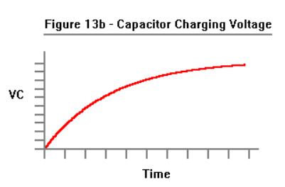
Without going through its derivation, the formula is:
VC = V * ( 1- e**(-t/R*C) )
The rise time for this RC circuit is defined as the time it takes for VC to reach 63.2% of its final value.
This number wasn't chosen arbitrarily.
When t = R*C,
VC = V * ( 1-
e**(-t/R*C) )
= V * (1-e**(-1) )
= V * (1-0.368)
= V * 0.632
(The value R*C is called the Time Constant of the circuit.)
Therefore, we need a really good current source such as the one in Figure 14.
An ideal op-amp has infinite gain and its inputs require zero current. Since there is no current flowing into the negative input to the op amp, all the current through C will be the same as the current through R. Since the op-amp has infinite gain, the voltage across between op-amp's positive and negative inputs will be zero, assuming the op-amp's output is less than infinite. By referencing the op-amp's positive input to ground, the voltage at the negative input will be zero.
Therefore the current through R is Vin/R, which will be same current flowing through C, so we have a voltage controlled current source, and applying a step voltage at Vin will cause Capacitor C to produce a nice linear ramp at Vout. The circuit inverts the polarity of the input, so a positive voltage at Vin produces a negative ramp at Vout and a negative voltage at Vin produces a positive voltage at Vout. Officially, this circuit is an Integrator because the output is the sum (over time) of all the input voltages.
If we already have a current we can skip Resistor R.
As it turns out, most DACs produce a current output. However, because most DACs have a limited drive capabilty (and want to see a low circuit impedance) most DACs use an op-amp on their outputs.
The circuit for a DAC connected to an Integrator is shown in Figure 15.
Notice that we have also added two resistors. DACs require a reference voltage (or current). That's what R1 is for.
R2 is to provide the offset current to convert the Unipolar DAC to one that provides a Bipolar output, which is why, in all of Atari's schematics, it's called the BIP. This method was covered in the section on Digital Vector Generators.
By the way, the DACs used in the earlier sections were assumed to have voltage outputs in order to avoid unnecessary detail. If we wanted a DAC with a voltage output that did not integrate the values we would replace the Capacitor with a Resistor and end up with the circuit shown in Figure 16.

Referring back to Figure 15, we now have a DAC that produces a bipolar output current that is the product of
Digital Inputs (in two's complement) * Vref * K
where K is a constant that represents the conversion gain and depends on what's in the DAC.
This output current determines the slope of the ramp produced by Capacitor C.
We are almost ready to draw some vectors. The problem is in starting and stopping the ramp. If we don't do a good job starting and stopping the ramp, the vectors will look pretty bad.
If we give the DAC a digital input of zero, the output current will be zero and Vout will stay where it is. Unfortunately, the DAC takes too long to change its current for this to work. The DAC also produces glitches when it changes.
The method used in all of Atari's Analog Vector Generators (with the exception of TomCat) was to switch the DAC reference on and off.
In Figure 17 we have chosen Resistors R1 and R2 to scale the Reference Current for the DAC as well as the Bipolar Offset Current for the Op-Amp.
How well this method works depends on :
1. How well the turn-on and turn-off characteristics of the DAC match.
2. How fast the vectors are drawn. The faster the vector is drawn, the more time it spends in the turn-on and turn-off periods, and therefore the more noticeable the turn-on and turn-off periods are.
In BattleZone the vector drawing speed was slow enough that the vectors look good.
By the time we got to Star Wars, the vector speed (and monitor speed capability) had increased to the point where the vectors looked really bad. We kept devising circuits to match the turn-on and turn-off characteristics of the DAC but the Programmers just drew the vectors faster in order to get more of them on the screen.
There is another problem.
The charge stored in the capacitor is a history of all the charge that has ever been stored in it, including all the turn-on and turn-off mismatches. In other words, the errors keep adding up.
If allowed to continue, objects would not end up where they are supposed to be on the screen. Eventually, the outputs would drift completely out of control.
The simplest method, and the one chosen, was to periodically discharge the capacitor, as shown in Figure 18.
This was done with an LF13201 Analog Switch. Analog switches like the 4016 and 4066 require that the control signal have a range somewhat greater than the analog signal to be controlled. That means if you want to control a signal that goes between -10V and +10V the control signal must switch between (a little bit more than) -10V and +10V. If you are controlling it with a TTL signal, it means making a level translator. (Asteroids has one.) The LF13201 contains the TTL level translator. It's more expensive, but worth it.
Now, we need to talk about capacitors.
Capacitors are more complicated than you may think. Not all capacitors work equally well in this application. In fact, there are very few capacitors that are acceptable here.
There are several properties of capacitors at work.
One is Leakage. It's like there is a resistor across our capacitor that causes it to discharge all by itself. This would cause the position of the beam to drift to the center so it isn't where it is supposed to be. Leakage is a function of the type and quality of the dialectric used.
Another is Inductance which will make the response of the Integrator change according to the vectors we are drawing. The Inductance of a capacitor depends on the construction of the capacitor. For example, take a capacitor whose plates are made by taking two foil strips of conducting material (such as aluminum) with a dialectric between them and rolling them up with an additional dielectric so that adjacent layers don't short out. If the connections to the plates are made on only one end, the other end will have the entire length of the plates between it and the capacitor terminal. The length of the plates will have inductance. However, if the capacitor terminals are connected to each layer at the sides of the roll the distance of each segment of the plates will be much shorter.
This is shown in Figures 19a, 19b, 20a, and 20b. In the interests of
clarity I have shown only one plate.
Another property of capacitors is Series Resistance. Like Inductance, Series Resistance will make the response of the Integrator change according to the vectors we are drawing. Again, this is caused by the construction of the capacitor as well as the shape of the plates and the material used in the plates. A capacitor constructed as in Figures 19a,19b will have a higher Series Resistance than the one in Figures 20a, 20b.
By the way, the official term for Series Resistance is Equivalent Series Resistance (ESR) and is an important specification of capacitors used in high frequency switching power supplies. When the current that is charging and discharging the capacitor goes through the Equivalent Series Resistance it produces heat. The greater the ESR, the greater the heat produced. You can't escape Ohm's Law.
The final capacitor property we will consider is related the phenomenon known as Charge Redistribution.
To start with, when you charge a capacitor to a particular voltage, the charges stored in the dielectric do not uniformly distribute themselves throughout the dielectric; they favor the positive plate. After all, the charges are electrons which have a negative charge.
And when you discharge a capacitor, the charges do not immediately redistribute themselves throughout the dielectric. This is why, when you think you have discharged a capacitor, you can come back a short time later and a small amount of charge has magically reappeared. No, the capacitor has not been recharged by the atmosphere, or the aether, or by phlogiston.
I did the following experiment with a 1000uF 25V electrolytic capacitor. First I connected a DVM across it to verify that it was fully discharged and that the DVM was not injecting current into it. The reading was 0.000V .
Next I connected a 9V transistor battery across it, observing polarity. The reading was 9.38V (it was a new battery.) When I disconnected the battery the voltage began to droop very slowly due to capacitor leakage.
I shorted the capacitor for about three seconds, then removed the short.
The results are shown in Figure 21. It reached a peak of about 0.34
Volts after 30 minutes.
When we discharge the capacitor in our Integrator we want it really discharged. Some capacitors do better than others for reasons that are not clear.
Mylar Capacitors were used in BattleZone, but did not work very well in Star Wars, which had a faster drawing speed. The capacitors that worked the best for us in Star Wars were Polycarbonate Capacitors.
Polycarbonate is a clear and colorless amorphous thermoplastic notable for its high impact resistance. In addition to its use in capacitors it is used in glazing, safety shields, and CDs. (An excellent Web site for the properties of materials is http://www.goodfellow.com/.)
Polystyrene capacitors are also considered high quality capacitors but they worked poorly in the Integrator.
The properties of polystyrene are similar to polycarbonate but for reasons that are unknown the polystyrene capacitors exhibited problems that appear to be the result of charge redistribution.
Finally, the issues of Leakage, Inductance, and Series Resistance are not confined to the capacitor itself.
They can also be caused by circuit design and layout. The circuit layout can also screw things up if there is crosstalk from another signal trace.
It doesn't always end there, either. One time I was asked to look at
a prototype AVG board for another project which was producing really
nasty vectors. The digital circuitry had been checked and was ok. We
ended up unsoldering all the parts in the Integrator and connecting
them together off the board in the air. That fixed the problem and we
concluded that the material used in the PC Board was contaminated. The
next run of prototype boards was ok.
We can now start and stop a ramp whose slope is determined by a 10-bit digital word. We can also discharge the Integration capacitor to center the beam.
This is analogous to the Digital Vector Generator where we can start and stop a ramp produced by a Binary Rate Multiplier which clocks a counter that feeds a DAC whose output is deglitched by a Sample-and-Hold.
There are several differences.
1. The Digital Vector Generator produces vectors consisting of points at discrete coordinates. While the Analog Vector Generator has discrete values representing the length of a vector, the values in-between are continuously and infinitesimally changed (subject to the restrictions of living in a Quantum Universe). Thus, there is no stairstepping.
2. The Digital Vector Generator can set the position to any coordinate by loading it into the counter. The Analog Vector Generator can only center the beam and draw a blank vector to the desired position. (The ability of the Digital Vector Generator to load the counter was mostly unused since the fastest the XY monitors could move the beam was about the same as the fastest drawing speed.)
3. The Binary Rate Multipliers in the Digital Vector Generator require inputs in Sign/Magnitude form, while the Analog Vector Generator uses Two's Complement values.
4. The Counters in the Digital Vector Generator require different clock frequencies to make different X and Y values, while in the Analog Vector Generator the X and Y values automatically produce analog ramps of the proper ratio.
Since we are always working with changes in vector length, they are referred to as Delta values. Delta is the Greek symbol used to represent Difference and, if your character set supports it, is represented by the Greek symbol ) or * which is where we get the Latin letter 'd' .
At this point we are faced with some of the same issues for the Analog Vector Generator as we were with the Digital Vector Generator, namely, how fast to draw the vectors. This has already been discussed in the section on Digital Vector Generators.
Faced with the same insatiable need to feed data to the DACs we
turned to the same solution, the custom processor made out of SSI and
MSI having at its heart, the Vector Generator State Machine. The basic
theory of State Machines has also been covered in the section on
Digital Vector Generators.
The Vector Generator State Machine used in the Analog Vector Generator follows the same general form as the one used in the Digital Vector Generator. Some of the differences are due to the differences between the analog circuitry in the Analog Vector Generator and the digital circuitry used in the Digital Vector Generator.
Some of the differences are related to the type of game the Analog Vector Generator was designed to run.
For example, because the trio of games scheduled to use the new Analog Vector Generator were 3D games where the vectors are the result of 3D transformations performed during program run-time, vector normalization must also be performed during program runtime. Therefore, the Analog Vector Generator performs vector Normalization as part of its operation. (The trio of games consisted of Malibu Grand Prix, BattleZone, and Red Baron.)
Another feature in the AVG used in these games is a Window circuit that allows the programmer to set a window. Vectors that are drawn outside the window are blanked. This was used in BattleZone to keep game vectors out of the radar display.
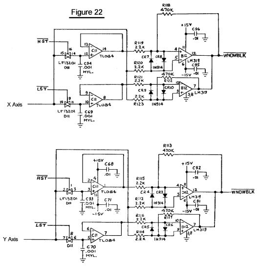
The way it works is quite elegant. (No, I didn't design it. I think Howard Delman did.) The programmer draws a vector (which can be drawn at zero brightness) to the desired position of the Lower Right Corner of the Window, and issues an HST Command. This operates Sample-and-Hold #1. The programmer then draws a vector to the desired position of the Upper Left Corner of the Window and issues an LST Command, which operates Sample-and-Hold #2.
The outputs of these Sample-and-Hold circuits are used with two sets of Comparators. One set of Comparators compares the current X position to see if it is Less than the X value of Sample-and-Hold #2 as well as Greater than the X value of Sample-and-Hold #1. At the same time, the other set of Comparators compares the current Y position to see if it is Less than the Y value of Sample-and-Hold #2 as well as Greater than the Y value of Sample-and-Hold #1.
If all these conditions are true, then we are inside the Window, and we refrain from blanking the vector.
The Window circuit is active all the time; it cannot be disabled. For a full screen display you simply set the Window to the full screen. This would generally be done anyway to keep the Spot Killer in the XY Monitor happy.
The Window circuit was used in BattleZone and Red Baron. No doubt it
would have been used in Malibu Grand Prix if the game had been produced.
Note that the Window circuit could have been used in the Digital Vector Generator.
One circuit that was used in the Analog Vector Generator that could not have been used in the Digital Vector Generator is the Linear Scaling circuit.
Referring back to Figure 18, in the Analog Vector Generator the current X and Y positions are contained in the Integrator Capacitors. If we change VREF we will scale the vectors beginning from that starting point; we do not affect that starting point. (In the Digital Vector Generator, changing VREF would also scale the starting point.) Thus, in the Analog Vector Generator changing VREF will change the linear scale of an object without changing its position.
Figure 23 shows how VREF is controlled using an 8-bit DAC.
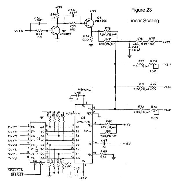
However, this method of linear scaling does not change the vector
drawing time, so that a vector that is linearly scaled takes the same
amount of time to draw as a vector that has not been, thereby wasting
vector drawing time. In order to scale an object over a large range,
the procedure is to use Linear Scaling down to 1/2; then bump the
Binary Scaling by 1 and restore Linear Scaling to 1.0 . (Binary Scaling
does adjust the vector drawing time.) This combined use of Linear
and Binary Scaling was used in Star Wars to blow up the Death Star
along with one other trick that will be explained later.
The final part of the Analog Vector Generator circuit, which was
used in all of the XY games, selected either the regular X and Y
signals or inverted versions of the signals. Sometimes it was just a
jumper on the board; sometimes it was under software control. This
allowed maximum flexibility in doing cocktail games where players
sitting across from each other took turns or games in which the monitor
was viewed through a mirror.
BattleZone was the first game to earn $500/week on field test. The company gave a party to commemorate this accomplishment. The game was hit of the Amusement and Music Operators Association (AMOA) show in the Fall of 1980 and was released in November 1980. (There was another game at the show that attracted very little attention at the time called Pac Man.) BattleZone sold about 25,000 units.
Red Baron was released in May 1981. It didn't do quite as well as BattleZone; it sold about 300 units. One of those units was in an airport when Wild Bill Stealey and Sid Meier played it and decided they could do better, so they went on to found Microprose.
Malibu Grand Prix was a driving game where you drove around a track.
It was loosely modeled after the Malibu Grand Prix go-kart driving
centers owned by Warner Communications, Atari's parent at the time. The
game was fun to drive; the problem was that as you better at it your
playing time went down. In a desperate attempt to salvage it, it was
given Sprint steering, from the game of the same name. In a real car,
as long as the steering wheel is turned, the car continues to turn. In
Sprint steering, the position of the wheel determines the position of
the car. It's ok (kinda) in a third person game like Sprint. In a First
Person game it's a disaster. Malibu was canceled shortly thereafter.
BattleZone and Red Baron were the first to use the Analog Vector
Generator. Starting with them we used a new DAC, the AM6012 by AMD.,
which was used in all of the Analog Vector Generators until TomCat.
Towards the end of TomCat, AMD stopped making the part. Fortunately,
there was another part, the DAC32HP made by Precision Monolithics Inc.
(PMI). Normally the Components Group evaluated parts to be added to the
Approved Vendors List (AVL) but since this was an especially critical
part I was asked to evaluate it, which I did, and gave it my blessing.
Later, Analog Devices acquired PMI, and they still make the DAC312HP.
The Data Sheet for the DAC312 is here (PDF 270KB).
Like the AD561J used in the Digital Vector Generator, the DAC312HP is generally considered difficult and expensive to find. And, like the AD561J, the DAC312HP can be purchased through Analog Devices' Web site (www.analog.com). The DAC312HP costs $6.75 (1's), $5.40 (25's), and $4.50 (100's). (PDF 87KB).
BattleZone and Red Baron both used another item of some interest, the Math Box, which did the arithmetic for the 3D math (multiplies, adds, and divides). The Math Box was built around the AMD 2901 Bit Slice which contained an Arithmetic/Logic Unit, a 16-deep dual port RAM, two registers, and a multiplexer. Each one was only 4-bits but had hooks so that it could be expanded. Four were used to produce a 16-bit machine and they were controlled by another State Machine. The Math Box hardware was designed by Dan Pliskin and programmed by Mike Albaugh. At one time Bit Slices were very attractive to people designing their own computers but have largely been replaced by FPGAs, sometimes implementing the 2901 architecture.
The working title for BattleZone was First Person Tank and then Future Tank. At one time it was to be called Moon Tank. The BattleZone team was as follows:
Project Leader: Morgan Hoff
Programmer: Ed Rotberg (Game Play, also the tank treads)
Hardware Engineer: Jed Margolin (3D algorithms, Object Digitization, Hardware Sounds, "Moon")
Technician: Doug Snyder (also hardware
design)
Bit Slice Math Box: Mike Albaugh and Dan Pliskin (For his work Albaugh received U.S. Patent 4,404,629 issued 9/13/83 Data Processing System With Latch For Sharing Instruction Fields)
Analog Vector Generator Design: Howard Delman
Design of 3D Objects: Harry Jenkins and Roger Hector
Volcano: Owen Rubin
Moon : (me). At the time, the game was going to be called Moon Tank which meant that the object in the sky would be the Earth, so I looked in my Almanac and used the East coast of Australia as a model.
Radar: At one of the early game reviews, Gene Lipkin objected to the radar because it looked like the radar in Subs. Since Subs had not been a successful game, Gene was afraid people would associate the radar with Subs, thereby dooming Battlezone. To give it a different appearance, Ed changed the radar so that it scanned from side to side. It looked so dumb that Gene relented and allowed us to restore the original radar.
Engine Sound: (me). I used two counters with slightly different counting periods and summmed several outputs to produce a somewhat disreputable waveform. Since the counters had different periods they produced a beat note when summed. As the frequency of the counters was increased, the beat note also increased. This is what makes the engine throb. The clock was generated by a 555 and had only two frequencies. To control the frequencies I used a circuit to shift the 555's threshhold voltage. This was done with a slow ramp so that the engine sound changed smoothly changed speeds.
Other BattleZone facts:
At one time, early in the game's development, it was configured to permit two people to play head-to-head on one monitor. This was made possible by the Window Blanking circuit. The two-player version was dumped, possibly because the resulting screen size for each player was considered too small.
Battlezone was the first game to use a new development system: the Blue Box and White Box duo. The Blue Box was programmed in Forth and controlled the emulator/analyzer in the White Box. It also had an external 8" floppy disk drive as well as a serial port for connecting to the VAX. Unfortunately, it did not have a full featured editor/assembler. Editing/assembling/linking was originally done on the department's PDP11 Model 20s which placed the output file on an 8" floppy, which could then be loaded by the Blue Box.
Later, when we got the first VAX, the Blue Box could be used as a terminal and the VAX was used to edit, assemble and link the program, and the output could be downloaded into the Blue Box/White Box.
The Blue Box was especially fond of reporting Comm Error 60 when it got confused, which was often.
The Blue Box/White Box replaced the Black Box. With the Black Box
system, programed were edited, assembled, and linked on the PDP11 Model
20s, and a paper tape was produced. The Black Box used its Paper Tape
reader to load the program.
A few months after BattleZone was released we received a letter from a fan who knew someone who knew someone who had seen someone drive up into the mountains, find a castle, and get a zillion points.
It was news to me. And to Ed.
There was also a rumor that U.S. Army Recruiters used to hang around arcades and when they saw a likely-looking candidate playing BattleZone, would go up to him and ask, "How would you like to drive a real one?"
And finally, I want to mention Doug Snyder. Although he was
officially a Technician, he was a skilled hardware engineer. Eventually
he was promoted to Hardware Engineer and went on to design the Slapstic
Security IC, Growth Motion Object Hardware (used on the G1 board in
Hydra and Pit Fighter), as well as many other things. (Between Morgan,
Doug, and Howard, there wasn't a whole lot of hardware for me to design
in BattleZone.)
Tempest came out in October 1981 and added color. However, the game used the Wells-Gardner Color XY Monitor which did not have pincushion correction, so the pincushion correction circuitry was put on the Tempest PC Board. (This is covered in The Secret Life of XY Monitors.)
Tempest did not have the Window circuit, either because it was not needed by the game or because the board space was needed by the pincushion correction circuitry.
Tempest also used the 2901 Math Box for its 3D calculations.
Space Duel (February 1982) had the pincushion correction circuitry,
no Window circuit, no Math Box, and not even Linear Scaling. But it did
have something new: the AVG Gate Array, formally known as the Vector
Generator Stack and PC Processor. This was a gate array designed
by Dean Chang that contained the Program Counter, the Memory File
Stack, and the Stack Counter. Figure 24
shows what's in it, followed by the specification of the part. All XY
games produced after Space Duel had the Gate Array.
Gravitar (June 1982) had Pincushion Correction and Linear Scaling.
Black Widow was released in February 1983. I don't have a manual so
I don't know what's in it.
Quantum (November 1982) was not designed by Atari. It was one of the two games that came out of a legal settlement with General Computer Corporation of Cambridge, Mass. (The other game was Food Fight.) GCC got into the game business by reverse engineering the Missile Command program and coming out with a new and improved version. Unfortunately, their version still said 'Missile Command' and they got sued. (They were also accused of including some code from the original Missile Command in their ROMs.) Fortunately for them, Atari had an amazing habit of suing people, winning the lawsuit, and paying the (losing) defendants a bunch of money.
Quantum used a 68000, which those of us at Atari had wanted to use ever since it had come out, but were not allowed to because "it was too expensive" and "the 6502 was good enough" and we didn't have a development system for it. Grrr.
Quantum used the Vector Generator Gate Array, Pincushion Correction, and Linear Scaling. My interest in Quantum came when I started TomCat, which I will cover more fully later.
I was at AMOA the year Quantum made its debut. In fact, my booth
duty was with Quantum. Quantum was not exactly ready for Prime Time and
had a habit of crashing about every 12 minutes, so every 10 minutes I
would casually reach into the Quantum cabinet and reset the machine.
After Quantum was released we were eventually allowed to use the 68000.
(We used a variant of the 68000, the 68010)
Unfortunately, the move to the 68010 did not happen in time for me
to use it in Star Wars.
The Star Wars game came about because I wanted to do a 3D space war game. I mean, I really wanted to do a 3D space war game. It's why I went to work for Atari. Even before going to Atari I had already worked out the math for 3D that did not use Homogeneous Coordinates. The use of Homogeneous Coordinates just gets in the way of understanding what is really going on in 3D.
At my job interview I handed my interviewer (Dave Stubben, the Chief Engineer of Coin-Op) a game description of what I wanted to do. He said that he couldn't promise me that I would be assigned to any particular game. Nonetheless, when I was offered a job, I accepted it. Atari brought me out to Sunnyvale for a second trip so I could find a place to live. (I rented an apartment.)
I almost didn't get to Atari. It was Friday afternoon and the Movers were scheduled to come on Tuesday (Monday was New Years Day). I received a call from Atari's Director of Personnel (Phyllis Pearson). It seems Atari was in some kind of financial difficulty and had just laid off some engineers in the Consumer Division and it had been decided that my job should go to a laid-off Consumer Engineer. I explained that the Movers were scheduled to come on Tuesday, that the day after that I would have no place to live because I had already given up my apartment, and that I was in some financial difficulty myself from having rented an apartment in Sunnyvale. Phyllis said she would see what she could do, and later called back with the good news that they had decided that I was too far in the pipeline for them to flush me (or words to that effect).
I arrived at Atari in early 1979. The first game I was assigned to was Sebring, a driving game that was started ostensibly to use up a supply of old 25" color monitors. It was a sitdown game with a curved projection mirror made from silvered Plexiglas. Since the curve was set by stuffing a flat mirror into wooden guides, it was optically rather poor, and gave the player a headache. (This was the Mechanical Group's idea of how to make a cheap mirror.) The monitor was mounted on top of the cabinet.
Sebring was a first person game, using the stamp hardware that was used back then. I was the Hardware Engineer, Paul Mancuso was the Technician, and the Game Designer/Programmer/Project Leader was Owen Rubin, one of the great game designers. Owen came up with several innovations that were copied by later generations of driving games:
1. The player drove around a circular track; the hardware made it look like the objects that were farther away were smaller.
2. The player saw the front of his own car, which shook as the car was driven.
3. There were other cars on the track which the player had to get around.
4. The player started the game by starting the engine, which started with a bang, a hardware bug that we liked, so we kept it in.
Paul and I put a large speaker in the front of the seat, between the player's legs which gave the player a nice buzz from the engine sound. Years later, this feature was used by others, who patented it. (Grrr).
Although Sebring did well in field test, it was cancelled because, supposedly, the vender who made Atari's cabinets didn't want to make it. (Perhaps he wanted too much money.)
I believe there was only one prototype, last seen in Paul's possession. I wonder if he still has it.
Another early game was Tube Chase in its XY incarnation. Owen Rubin was the programmer on that one, too. The problem with doing Tube Chase in XY is that there was no way to do hidden line removal. which makes traveling through a tube confusing. Later, Tube Chase was done on Dave Sherman's new circle generator hardware, which drew circles without a bit map. Although Owen finished the game and it did ok on Field Test, by then Atari had several games ready that were considered really hot, so Tube Chase was put on hiatus. Later, it was licensed to Centuri who produced it as Tunnel Hunt. Owen took to referring to Tube Chase as "The Game That Wouldn't Die."
Then came BattleZone, which used a stripped-down version of the 3D math I had developed for my space war game.
Finally, I was given permission to start my game, which I called Warp Speed. Greg Rivera was the programmer; Ed Rotberg was the Project Leader. Then Ed , along with Howard Delman, left Atari and started their own company Vidia, which was later bought by Nolan Bushnell and folded into Sente.
Greg and I needed a project leader and selected Mike Hally. Usually the project leader selects the team. In this case the team selected the project leader.
We went through several technicians until we got Erik Durfey. (It appears that the previous techs didn't want to spend their time on a game that was a guaranteed loser.) Later we acquired an additional programmer, Norm Avellar
At some point Atari Consumer started working with Lucasfilm. I suggested to Dave Stubben that Warp Speed would be a good platform for a Star Wars game. Apparently, he agreed.
Star Wars was field tested around May 1983 and went into production in July. The Star Wars AVG had Linear Scaling and the AVG Gate Array. Here is the Vector Generator Instruction list (PDF 49KB ).
There was something different about the AVG, though.
In order to have the Death Star explode the way we wanted it to, it wasn't enough to draw lots of concentric circles. We wanted to defocus the beam to fill it in. We briefly considered adding a vacuum tube to the monitor to control the Focus Voltage. Fortunately, the lead time for the part was too long. So what I did was to give the Vector Generator the ability to overdrive the monitor's color inputs. Overdriving the inputs causes the CRT to draw more current than it normally uses and drags down the High Voltage., which changes the normal ratio of Focus Grid voltage to Anode voltage, which defocuses the beam. This relationship is explained in The Secret Life of XY Monitors.
Star Wars is different from previous XY games in other ways as well.
The Main Processor is a Motorola 68B09E which I chose because its instruction set is slightly more advanced than the 6502 and because I couldn't use a 68000.
There are three LEDs on the PC Board solely for diagnostic purposes, which Greg and Norm used during development to indicate when certain events were taking place. I think the game was released with them still programmed.
There is a hardware Linear-Feedback-Shift-Register (Pseudo-Random Number Generator) for generating random numbers for star creation. While this function could have been implemented in software, it would have eaten up processor time.
The amount of math that was needed for the game was more than could
be done with the Bit-Slice Math Box used in BattleZone, Red Baron, and
Tempest, so I designed a new one. The basic function in the 3D math we
used is a matrix multiply of the form:
This can be broken down into three operations of the form:
X' = AX * (X-XT1) + BX
* (Y-YT1) + CX * (Z-XT1) + XT1
The basic operation is a Multiply/Accumulate with a Pre-Multiply Subtract of the form:
ACC = ACC + (A-B) * C Equation 2
Although there were some very fast bipolar multiplier/accumulators available from TRW, they were much too expensive (and Star Wars was designed before the invention of the DSP), so I settled for 74LS384 Serial Multipliers and 74LS385 Serial Adder/Subtractors.
The 74LS384 multiplies an 8-bit word multiplicand by a 1-bit multiplier. It produces a 1-bit product and keeps a running sum for multiplying the next most-significant-bit. By using two 74LS384s we can multiply a 16-bit multiplicand by a 1-bit multiplier. The 74LS385 Serial Adder/Subtractor operates with two serial bit streams, adding with Carry or subtracting with Borrow (however it is set up) and producing a 1-bit result while saving the Carry (or Borrow) for the next most-significant-bit.
With a 12 MHz clock, Equation 2 takes 2.58 us to perform. This is for 31 clocks. Normally it would be 32 clocks to get the entire 32-bit result of multiplying two 16-bit numbers. Why there is one less clock relates to how we represent the number 1.000. I think it will take another article to explain it.
Although a TRW Multiplier/Accumulator would do it in 50 ns, the Bit-Slice Math Box would probably take10 us (I'm guessing).
The basic block diagram for the Multiplier/Accumulator with
Pre-Subtract (the MAC) is shown in Figure 25.
For controlling the Multiplier/Accumulator and keeping it supplied with data I designed a simple Data Pump. Although it is microprogrammed, it is not a State Machine.
We start with a PROM to provide the various strobe signals to load the shift registers and the parallel input to the Multipliers and to start the counter to provide the correct number of serial clocks to the MAC.
The PROM is programmed to provide the desired set of microinstructions starting from a selected address. After each micro-instruction a counter increments the PROM address. The last instruction in the sequence sets the MHalt flag which stops the process and alerts the 68B09E that it has finished its task.
The programmer selects different programs by selecting the appropriate starting address in the PROM.
The data for the MAC is stored in a completely separate memory (a RAM) that the 68B09E writes to when the MAC is halted. The results of the MAC are not stored in the RAM; the 68B09E reads the contents of the Accumulator directly.
The address for the RAM comes from a counter that can be set by the 68B09E. After each program this counter is automatically incremented to make it easy to perform an operation on blocks of data. An example is when we transform the points that make up an object (like Darth Vader's ship).
The block diagram for the Matrix Processor Controller is shown in Figure 26.
The Divider for performing the Perspective Divide is a totally separate unit. It is unsigned and is of conventional design.
Because they are separate, the programmer can perform Perspective Divides while waiting for the Matrix Processor to deliver the next transformed point.
I designed the Matrix Processor specifically to perform Equation 1. However, Greg kept figuring out how to make it do more things, such as Dot Products and Cross Products.
The 3D math that Star Wars was capable of performing allowed any object (and the observer) to be in any orientation. However, it was decided that players might be confused by being approached by an upside-down TIE Fighter, so they were forced to be right-side up most of the time.
I want to mention the Sound Board, which had its own processor (another 68B09E). Although other companies had done games where the Sound System had its own processor, this was a first for Atari.
Star Wars didn't start out with a separate processor for sounds. In fact, in the first prototype board there was only one 68B09E that did sounds as well as the game. However, well into the project Greg and Norm absolutely needed more ROM space for the game and the 68B09E was completely full. I jokingly suggested that the best way to give the game more ROM was to add a separate processor for sounds. They liked the idea; so did Mike. And so did Rick Moncrief, the Director of our group. So, I came up with a Sound Board with its own processor. And, as long as I was at it, I put in four Pokeys. (The Sound System always had the Texas Instruments TMS5220 Speech Synthesizer.)
At one point I suggested we modify the Sound Board so it could accept either a Quad Pokey or four Pokeys. I was told by Engineering Management, "No. We don't want people to know that a Quad Pokey is four Pokeys."
I also put in something else; an image expander, also known as a stereo faker. The way this works is that you take your mono signal, delay it, and use it as a difference signal that you separately add to the original signal to produce the Left Channel and subtract from the original signal to produce the Right Channel (or vice versa). The result is to randomize the phase which your ears interpret as, "Where the Hell is that coming from?"
Unfortunately, the speakers in Star Wars are mounted too close together and too far from the Player to produce much of a stereo effect. It sounds great in headphones, though.
At some point, Rick hired Earl Vickers to do sounds and speech
development. Up until then, the game programmers were responsible for
sounds, which they generally hated doing, so usually the programmers
would use Pokey sounds that had already been developed. That's why, for
many years, most of Atari's games sounded alike. The other game groups
decided that having someone just do sounds was a good idea so Earl
became the nucleus of a completely separate Sound Group that did sounds
for all of the games. Well, almost all of the games. Hard
Drivin'/RaceDrivin' was an exception. I will leave that story for
perhaps another time.
There is a design on the Sound Board artwork that is the signature of the PC Board designer, Denny Simard. Denny was experienced in doing analog boards and was a member of our group, as opposed to being in the PCB Group. He was a nice guy and also looked *exactly* like Frank Zappa.
Unfortunately, he only got to do a few boards before being caught in
one of the first Great Layoffs. [Which became "Reduction-In-Force" and
then "Downsizing"].
The control yoke for Star Wars was a downsized version of the control from Army BattleZone (minus the palm switches), which came directly from an actual Bradly Fighting Vehicle. (It was the Gunner's control.) You might have noticed that the centering of the Star Wars control yoke is funny at times. Star Wars originally used a Pokey to read the pots. At that time, people either made their own A/D converter with a counter, a comparator, and a ramp, or they used Pokey. The Pokey was a full custom IC designed for the Atari 800/400 to read pots and keys, which gave it its name, POts and KEYs. There was some room left over so they put in some crude square wave sound generators as well as a UART. Unfortunately, Pokey does a really awful job of reading pots; it is guaranteed to produce occasional wrong values. The software to deal with it is pretty nasty. After Greg Rivera brought this to my attention I took the daring step of actually putting in a real A/D (Gasp!), the ADC-0809. Unfortunately, many people continued to use the original code to treat the A/D values as though they had come from a Pokey. Like Greg. That is why the Controller in Star Wars keeps getting recentered, usually badly.
During an early phase of development, when it was still Warp Speed, we tried a two-player game by connecting two monitors to the hardware with a circuit to allow the software to independently blank the video to the monitors. The vectors were still drawn on both monitors, but you didn't see them on the blanked monitor.
There was still only one hardware system, so it could only calculate and draw half as many vectors for each player, but it was an instructive experiment. It turns out that if you fire the laser (phasor, photon torpedo, photonic cannon, or whatever) by pointing the ship, the best strategy is to sit and fire at the other ship. If you try to maneuver, you have to point away from your opponent's ship. When you point away from your opponent's ship, you can't fire at it. (Well, you can but you won't hit it.) Therefore, the ship that tries to maneuver, loses. It wasn't much fun.
At one point during the development of the game there was a Thrust
Control. However, the faster you could pilot your ship, the less game
time you got, so Mike and Greg took it out. The Thrust input is still
shown in the schematic.
At one time, the game had a joystick instead of the Flight
Controller. The people at the focus group were confused about which way
they were supposed to move the stick and we were able to use that to
justify the higher cost of the Flight Controller
Star Wars joke: "No, No, No, " exclaimed Obi Wan at dinner one
evening, " Use the Fork, Luke!"
When Star Wars came out, it was the Number #1 Game until Dragon's Lair came out. Unfortunately, Dragon's Lair came out two weeks after Star Wars.
Nonetheless, we sold around 15,000 Star Wars games with a margin of
about $1,000 per game for a total of about $15M. The period 1983-1984
was especially tough for Atari. We referred to it was "Going
Supernova."
Warner Communications gave Atari Consumer to Jack Tramiel for $70M in paper which they later tore up. After Jack Tramiel had built up Commodore from a small manufacturer of business equipment and turned it into a successful maker of personal computers, he had a disagreement with the chairman of the company, and quit. He then turned around and offered to take Atari Inc. off of Warner's hands. Two things to note:
1. Warner retained a minority ownership
2. Tramiel didn't want Coin-Op because he didn't think games had any future.
We (Coin-op) were given to Namco in payment for the royalties that Atari, Inc. owed Namco in royalties for Consumer's Pac Man game.
Toward the end of that period we were told that Atari Games (our new name) had just barely broken even.
Presumably, that's why we hadn't been shut down or otherwise gutted.
Breaking-even included the $15M from Star Wars.
After Star Wars, the remaining XY games that were produced were Major Havoc and The Empire Strikes Back.
Major Havoc (November 1983) had Linear Scaling, a Window circuit that operates on the Y Axis only, the AVG Gate Array, and two 6502 processors.
The Empire Strikes Back (March 1985) was a kit for Star Wars.
It featured the Slapstic for expanding the 64 KByte address space of the 6809 as well as providing security. Slapstic was a small semi-custom IC and had three security levels: Simple, Medium, and Complex. Most games used the Simple level because it was the easiest for the programmer to deal with. Most programmers preferred to spend their time working on the game, so Slapstic security was usually left until the night before the ROMs had to be released for production.
The last game to use Slapstic was Hard Drivin'/Race Drivin'. After
that, Slapstic was scrapped and replaced with a GAL6001 PLD which had
buried states that were not brought out to the outside world, making it
difficult to analyze the states programmed into it. It was also
supposedly secure once the security bit was programmed. Unfortunately,
the GAL6001 were cracked even more easily than the Slapstic in Simple
Mode.
I have talked about TomCat in a previous article TomCat - Atari's Last XY Game which also contains screen shots of the game.
This is about the hardware.
I have scanned the schematics and put them into a printable form (PDF 1.8MB). There is also a picture of the board (526KB), one of only two boards known to exist. The picture was taken by Scott Evans and comes from the TomCat article.
TomCat used a 68010 running at 6 MHz. The 68010 was a terrific processor. (I still like it.)
The 68010 is a 32-bit machine internally, with a 16-bit bus to the outside world. (There was another variant, the 68008 which was 32-bits inside with 8-bits to the outside world.)
One of the nice things about the 68010 was that it had a small cache which was large enough to hold the following instructions:
* Initialize Register2
* R1 = Source Address,
* R2 = Destination Address,
* D1 = # of words to move
loop: MOVE.W (R1)+,(R2)+ *
move the word whose address is contained
*
in Register R1 to the address contained
*
in Register R2, increment the contents
*
of Register R1 and Register 2
DBNE D1,loop * If the contents of
Register D1 are not zero,
*
decrement the contents of Register D1 and
*
branch to loop
This allows you to move data around faster than with the vanilla 68000 since it does not have to spend time repeatedly fetching the instructions from external memory.
The 68010 also executed the Divide instruction faster than the 68000. (I guess they fixed the microcode.)
Unfortunately, the 68010 never caught on and was always more expensive than the 68000.
The 68010 presents special problems when interfacing it to the AVG, or any other processor for that matter.
The 6502 has a synchronous memory bus where the master clock is divided into two phases (Phase 1 and Phase 2). The address is always generated during Phase 1 and all memory accesses take place during Phase 2.
The 68010 has an asynchronous bus where the number of clock phases (and the phases where memory is accessed) depend on the instruction. This is a consequence of the 68010 being a microprogrammed machine with its own state machine, while the 6502 is a random-logic machine. If you have read the previous section of this article on the Vector Generator State Machine you know exactly what the difference is.
Because it has an asynchronous bus, the 68010 requires that the hardware acknowledge that it has completed the bus transaction by asserting a Data Acknowledge signal (/DTACK). Until /DTACK is asserted, the 68010 will just sit and wait.
To deal with the problems of an asynchronous bus Quantum used a rudimentary circuit to generate Wait states for the 68000 so it wouldn't interfere with the Vector Generator State Machine when the Vector Generator State Machine was accessing data from the Vector Memory it shared with the 68000. As I recall, there were times when the 68000 stalled the Vector Generator when it didn't need to, and there were times when the Vector Generator stalled the 68000 when it didn't need to, either. To be fair, it's a difficult problem because the 68000's asynchronous bus may start a memory access in the middle of a Vector Generator access.
I felt I could do better.
In addition to /DTACK, the 68010 provides three outputs (F0, F1, and F2) that tell the hardware where the 68010 is in its execution cycle.
I decoded these signals so I would know exactly where the 68010 was in its execution cycle.
I also decoded the Vector Generator state so I would know exactly where it was during its execution cycle.
Then I used a PROM to decide who would get the memory and who would get stalled depending on who was where.
The 68010 state decoding is shown on Sheet 2A. The Vector Generator state decoding is shown on Sheet 9B. (It produces the signals VG-STALL and /VG-DTACK.)
I later used a variant of this method in Hard Drivin'/Race Drivin' so its 68010 could talk to the TMS34010 Graphics Signal Processor.
On to the Vector Generator.
The boards that were made contained the same basic Vector Generator as the one used in Star Wars. However, I modified one board in a special way that dramatically improved the quality of the vectors.
The original circuit is shown in Figure 18 and is reproduced here as
Figure 27. The vector is started and stopped by turning the DAC
reference on and off.
In the new circuit, shown in Figure 28, the DAC is on all the time. It is the connection between the voltage produced by the DAC and the input to the integrator that is turned on and off. (I am using the symbol for an analog switch.) A series-only or parallel-only switch does not work because of leakage in a series switch and non-zero resistance in a closed switch. Combining the two is the solution. The inverter causes one switch to be off when the other is on, and vice versa. (This is called an 'L' Switch.) Note that I have converted the DAC output current into a voltage before applying it to the 'L' Switch. In the actual circuit shown in the TomCat schematics on Sheets 12A and 12B there is an additional potentiometer on each axis to null out any offset to the integrators. The LF13201 analog switches turn on and off faster than the DAC, producing vectors with sharply defined end points.
Next is the Game Link.
I had always wanted to link games together. I even described it in the game description I brought to my job interview. In Star Wars I brought the Pokey's Serial I/O Ports out to the edge connector, hoping to get people interested in linking games. It didn't happen. So I did it in TomCat.
The TomCat Game Link is a 16-bit interface with full
handshaking. See Sheets 7A and 7B.
My best work on TomCat, though, is probably what I did with the TMS32010 Digital Signal Processor (DSP) that had only recently been brought out by Texas Instruments. Although it wasn't the first single-chip DSP (that honor goes to the NEC uPD7720), it was the most successful. (As a result of Texas Instruments' success with DSPs they would eventually dump many of their other product lines such as DRAMs and EPROMs in order to concentrate on DSPs.)
I used the TMS32010 for performing the 3D math calculations.
The 32010 had a 200ns instruction cycle time and most of their
instructions required only one cycle, including the Multiply/Accumulate
instruction.
The Multiplier was 16 x 16 bits with a 32-bit Acculumator, and all this in 200 ns! This was a gigantic leap forward compared to the Bit-Slice Math Box and the Star Wars Matrix Processor.
It also had a 0-15 bit barrel shifter, so you could shift anywhere from 0-15 places in one instruction cycle.
The DSP had 288 bytes on on-chip RAM and was available with 3K Bytes of on-chip (masked) program ROM or it could use external memory.
I used external memory.
And that presented a problem.
It seems that Texas Instruments had neglected to consider that someone might want to use the TMS32010 with a Host Processor sharing memory with it.
There was no way to stall the TMS32010. And even worse, Texas Instruments specifically warned that the contents of the internal RAM were not guaranteed to stay put when the device was given a Hardware Reset.
I could have used a parallel interface, but that would have slowed down the data transfer more than I wanted.
The TMS32010 had one saving grace, a Conditional Branch instruction that tested the state of an I/O pin (the BIO pin). The instruction was BIOZ <address> which would branch to <address> when the BIO pin was low.
So here's what I did.
I used RAM for the Program Memory with buffers that could connect it to either the 32010 or the 68010.
I then decoded the 32010's address bus to set a flag when the 32010 address was in any of its first four memory addresses (addresses 0-3).
When the 32010 was in any of the first four memory addresses I switched the buffers to disconnect the 32010's address and data buses from the Program RAM (giving it to the 68010) as well as switching the 32010's data bus to a set of buffers hardwired to produce a BIOZ 0 instruction. Therefore, when the BIO pin was low and the 32010 was at one of the first four memory addresses, it would branch to address 0 and stay there until the BIO pin (controlled by the 68010) was released.
I chose the first four addresses because the 32010's Reset vector was at address 0.
The way it worked was that the 68010 started out by setting the BIO Pin and resetting the 32010, sending it to address 0 where it would 'stick.' The 68010 could then talk to the Program Memory, setting up program code and data.
When the 68010 released the BIO pin, the 32010 would cease branching to address 0, would breeze past addresses 1, 2, and 3, and get to address 4 which would reconnect the Program RAM to the 32010.
The 32010 would then start executing the program in the Program RAM starting at address 4.
Each program would end with a branch to address 0, where it would 'stick', alerting the 68010 that the program was done.
The 68010 was then free to access the Program RAM in order to read the results of the program and set things up for the next program.
In practice, several programs were downloaded into Program RAM during initialization so the programmer (me) only had to place a Branch <address> instruction at Address 4 to call the desired program.
It worked out very well.
I later used the TMS32010 in Hard Drivin', but only on the Sound Board. By then, Analog Devices had come out with a DSP that was better suited for doing 3D calculations (the ADSP-2100).
I also used the TMS320P15 (a TMS32010 with an on-board EPROM Program Memory) in Race Drivin', mostly to provide security. I supported another team's project using the TMS320P15 for security. The TMS320P15 was supposedly hack-proof once the Security Bit was set. It wasn't. The reason I know is that in that project I put in an undocumented program that sent out the Atari copyright message in Morse Code. Because of the DSP's speed it could be received by just placing a standard AM radio near the PC Board. The program was called only by grounding an innocuously unused I/O pin during Reset. When Atari received a counterfeited game to examine, I placed an AM radio near the board, grounded the aforementioned I/O pin, gave it a Reset, and heard my Copyright Message on the radio.
The name of that game was Road Riot.
There is something different about XY. Perhaps it is because an object is completely drawn before moving on to the next one, while in a raster game objects are drawn in pieces at different times on different scan lines.
It may simply be nostalgia; the old memory of when XY games had so much better resolution than their raster brethren.
And, since there haven't been any new XY games in 16 years, we may associate XY games with that period of our lives.
Some people are interested in XY games the same way other people are interested in old radios. Some people are purists; they would rather have a non-working old radio than use a few modern parts to get it going.
Some people are perfectly happy with a modern replication; they are in love with the idea of an old radio. Either way is fine. The nice thing about a hobby is that you don't have to justify it.
There are several possibilities for someone wanting to continue the development of XY technology.
1. Put the entire State Machine Vector Generator into a Field-Programmable Gate Array (FPGA). FPGAs are now large enough that you could probably include the vector memory as well. The downside is that FPGAs that are large enough to do this are available only in Surface-Mount Devices (SMDs) which require multi-layer PC Boards with solder masks. In prototype quantities these boards are several times more expensive than two-layer boards with no solder mash. SMDs also require specialized soldering equipment, which is also expensive. Finally, large FPGAs tend to operate only at 3.3 Volts, so that if it is necessary to interface them to 5 Volt circutry, some kind of level translation is necessary.
2. Before I ended TomCat, the next thing I was going to try was to replace the State Machine Vector Generator with a TMS32010 DSP. Today, there are much more advanced DSPs available such as the ADSP-2186 from Analog Device (www.analog.com). The ADSP-2186 is a fast (33 MHz) DSP with enough RAM memory on-chip to do the whole thing. All you need is the analog back end. It's even a 5 Volt part. One of the downsides is that it is an SMD part, The other downside is that Analog Devices has not make it easy to interface to other devices to it (like latches). Although the buses are brought out to the outside world, the signals are very fast and the address and data setup and hold times are difficult to work with.
3. Replace the entire State Machine Vector Generator with a Pentium-class PC. Just put the back-end circuitry (and a vector timer) on a PCI (or AGP) card. You would probably have to run DOS or Linux. Windows would be difficult to work with and might be too slow.
The back end I was referring to could be the one that ended up in TomCat, shown in Figure 28.
It could also be an updated version of the Digital Vector Generator. The AD561 was a 4 MHz DAC. Today, you can easily get a 30 MHz DAC. (Of course, you would need an equally fast Sample-and-Hold.)
A third alternative is something I have not completely worked out. Each axis has two DACs, two analog multipliers, an adder, and a Ramp. Referring to Figure 29, as the Ramp goes from 0 to 1 Volt, the 1-Ramp goes from 1 to 0 Volts, causing VOUT to smoothly transition between position X2 and position X1.
We start at position X2 when Ramp = 0 and 1-Ramp = 1. When the Ramp reaches 1, 1-Ramp will have reached 0, so we will have arrived at position X1. At this point we can change X2 for the next end point. We reverse the Ramp so when it reaches 0, we will end up at the new position X2.
The equation is: VOUT = X1* Ramp + X2*(1-Ramp) .
The creation of the Ramp is a major challenge. Assuming Star Wars
speeds (160 us across the 1024 pixel screen), it may have to go from 0
to 1 Volt in as little as 156 ns (1 pixel) or as long as 160 us (1024
pixels).
There is also the monitor problem. While most of the XY Monitor can be easily duplicated, the Deflection Yoke must be specifically designed for XY. You cannot use one designed for a TV.
Perhaps if we wait a little we will be able to make our own display from Light-emitting polymers (LEP). See Plastic display prototype proves inkjet technology, Electronic Products , April 2001, page 23. (Electronic Products)
XY might not be so dead after all.
In a Digital Vector Generator, each XY position comes from the output of a counter so the result is similar to what you would get by using a frame buffer. Since the Digital Vector Generator in Lunar Lander and Asteroids used 10-bit DACs we have a screen resolution of 1024 x 768. (We actually could use 1024 x 1024 but then the 4:3 aspect ratio of the CRT produces different X and Y scaling values.)
As a result, lines have the same stair-stepping that you get in a frame buffer.
So, considering the effort that was required to develop the technology (the XY Monitor as well as the Vector Generator) the question is, why did we bother?
The answer is, that in 1978 when the Digital Vector Generator was developed for Lunar Lander, memory was much too expensive for a frame buffer in a video game. The first game to use a frame buffer was several years in the future (Missile Command) and even then, it was low resolution. (It may have been 512 x 384, but I'm not sure.)
Even in 1980, the latest and greatest DRAM was 16K bits and cost about $4.80. A single 256 x 256 x 4 frame buffer would have required 16 devices at a cost of $74. Two frame buffers would have required 32 devices costing $148 just for memory, which was more than the cost allowed to manufacture the entire PC board. Two frame buffers of 512 * 512 * 4 would have required 128 devices costing $614.
Video games of the time used Motion Objects and Playfield ROMs.
Motion Objects was Atari's name for what others called Sprites. Since Atari invented the technology, the companies 'borrowing' it should have been honest enough to call it by its correct name. (A Sprite is just a Motion Object with the serial numbers filed off.)
The way a Motion Object works is that the programmer specifies a stamp (a picture) and a position on the screen. The hardware knows where the beam is (because it generates the sync) and pulls the correct data from the Motion Object ROM at precisely the right time. There is no frame buffer. Later, a line buffer was added to permit multiple objects to use the same Motion Object ROM. During Horizontal Sync, the hardware went through the display list and assembled the appropriate data for the upcoming line. Over the years the hardware evolved to permit more and more objects to share horizontal lines. Even so, there was always a limit on how many Motion Objects (or parts of Motion Objects) could exist on the same horizontal line.
Playfield ROM was just a picture burned into ROM that was scanned out. (Masked ROM was relatively cheap.) A later refinement was the Scrolling Playfield, which allowed the Playfield to be moved around.
Motion Objects and Playfields are what made the Atari VCS (later renamed the 2600) possible. The Atari 800 (and 400) used Motion Objects and Scrolling Playfields (implemented in custom ICs) as well as a frame buffer.
The hardware to do Motion Objects and Scrolling Playfields was used for quite a long time, even after frame buffers became common.
I expect that Motion Objects and Scrolling Playfields were used until it became impossible to compete with the graphics hardware developed for PCs, which is what is mostly used now in the (dying) coin-op industry.
But in 1978, there was almost no PC industry. For most people of that time, Lunar Lander and Asteroids were the most advanced interactive computer systems they could actually put their hands on..
The Analog Vector Generator got rid of the stairstepping produced by the Digital Vector Generator. It was first used in BattleZone (1981) and Tempest (later in 1981) added color.
These systems were also more advanced than what was available in home game consoles, not to mention the budding Personal Computer industry.
So, what happened? How did we lose our technological lead?
I think we lost our technological lead because we were so successful, and here's why.
The first 'video game' that I know of was developed in 1946. (U.S. Patent 2,455,992 Cathode-Ray Tube Amusement Device Thomas Goldsmith and Estle Mann). Although it used a sawtooth circuit it was essentially an XY game.
The first video game of the modern era (Computer Space) was invented in 1972 by Nolan Bushnell and Al Alcorn. Since the first microprocessor (Intel's 4004) was still in the process of being born, the game was a completely hardwired machine. Different operations were performed at different times according to the Counter used to produce Vertical Sync. The Motion Objects were stored in a diode matrix. The objects were created by stuffing the diodes in the appropriate holes in the PC board.
Computer Space was not very successful. The next game, Pong, was.
Even so, it didn't even register on the radar of the semiconductor companies.
Even when the semiconductor companies started making ICs for the Pong-type games for the home market, the semiconductor industry wasn't very interested in graphics.
When MITS developed the first
personal computer (the Altair 8800) in 1975 it used a front panel with
lights and switches. (There is a good article on the 8800 at www.vintage-computer.com/altair8800.shtml
.)
When Apple came out with the very successful Apple II, it had a frame buffer (hurrah!) but no hardware assist; the programmer had to laboriously (and slowly) manipulate the bits himself/herself.
When IBM came out with the IBM PC, it, too, had only a character generator. Other companies developed Frame Buffers for it, but again, with no hardware assist.
When Atari came out with its 400/800 computers, they had Motion Objects, Playfield Memory, and a Frame Buffer. It was a very advanced graphics computer (for its day) but Atari had to develop the custom ICs itself, because the semiconductor companies did not recognize the value of graphics.
The reasons why the IBM was successful in the personal computer business, but Atari was not, would take a book of its own. Part of it comes down to marketing. Atari's was bad; IBM's was good. After all, "No one ever got fired for buying IBM", even if IBM didn't design the product, or build it, or write the software for it.
However, because the IBM PC had an open architecture, other companies were able to build better and better graphics cards for it. Eventually these companies were successful enough to design their own graphics ICs.
Well into the 1980s, Atari Coin-op was still able to compete with PCs because
1) We were not hobbled by the PC's 80x86 processors. The first microprocessor that Atari used was MOS Technology's 6502, which was more capable than Intel's 8080. When we started using the Motorola 68010, it was more capable than the Intel 80286, and about par with the 80386 which came later.
2) Atari started designing its own custom and semi-custom ICs for its coin-op games.
Texas Instruments was the only company that made a serious effort to enter the PC graphics business with the TMS34010, which was a nice 32 bit processor with additional instructions for doing graphics.
TI failed in the PC graphics business, but I used the TMS34010 in the Hard Drivin'/Race Drivin' series of games. Even so, the TMS34010 was not fast enough to do enough polygons without a special trick I developed. Perhaps some day I will write about it.
At some point in the early 1990s, the demand for PC graphics became hot. People wanted the games on their PCs to be as good as the ones in the arcades.
The small companies making graphics cards for PCs became larger companies in an increasingly competitive industry. Because of the competition, many (or most) of these companies either failed or went into other areas, and their places were taken by other companies.
The reason Atari started designing its own graphics ICs was that it was the only way to get the ICs we needed. We were a games company, not an IC company.
We couldn't compete with companies whose only business was designing graphics ICs. At some point this included the entire hardware system, especially when you consider the large numbers of PCs made compared to the small number of custom hardware systems used by a shrinking Coin-Op industry.
One of the main things that fuels the demand for PC graphics is 3D games.
Although other companies made 3D games, Atari was the pioneer. For many people, their first experience with an interactive 3D game was BattleZone. A few years later it was Star Wars. Both were XY. Shortly afterwards came I, Robot, the first 3D polygon game. After that came the Hard Drivin'/Race Drivin' series.
Like I said, we were a victim of our own success.
There are worse things that can happen to a person.
Jed Margolin
San Jose, CA
April 22, 2001
Revised: July 21, 2001; July 20, 2003
________________________________________________________________________________________
Copyright 2001 Jed Margolin
Please send comments to: comments@jmargolin.com